Use the “summary” function to get summary statistics for all columns in the “mtcars” dataset.
Your final output should resemble the following:
#       mpg             cyl             disp             hp
#  Min.   :10.40   Min.   :4.000   Min.   : 71.1   Min.   : 52.0
#  1st Qu.:15.43   1st Qu.:4.000   1st Qu.:120.8   1st Qu.: 96.5
#  Median :19.20   Median :6.000   Median :196.3   Median :123.0
#  Mean   :20.09   Mean   :6.188   Mean   :230.7   Mean   :146.7
#  3rd Qu.:22.80   3rd Qu.:8.000   3rd Qu.:326.0   3rd Qu.:180.0
#  Max.   :33.90   Max.   :8.000   Max.   :472.0   Max.   :335.0
#       drat             wt             qsec             vs
#  Min.   :2.760   Min.   :1.513   Min.   :14.50   Min.   :0.0000
#  1st Qu.:3.080   1st Qu.:2.581   1st Qu.:16.89   1st Qu.:0.0000
#  Median :3.695   Median :3.325   Median :17.71   Median :0.0000
#  Mean   :3.597   Mean   :3.217   Mean   :17.85   Mean   :0.4375
#  3rd Qu.:3.920   3rd Qu.:3.610   3rd Qu.:18.90   3rd Qu.:1.0000
#  Max.   :4.930   Max.   :5.424   Max.   :22.90   Max.   :1.0000
#        am              gear            carb
#  Min.   :0.0000   Min.   :3.000   Min.   :1.000
#  1st Qu.:0.0000   1st Qu.:3.000   1st Qu.:2.000
#  Median :0.0000   Median :4.000   Median :2.000
#  Mean   :0.4062   Mean   :3.688   Mean   :2.812
#  3rd Qu.:1.0000   3rd Qu.:4.000   3rd Qu.:4.000
#  Max.   :1.0000   Max.   :5.000   Max.   :8.000
Exercise: 16-A
Use the “lm” function to create a linear model using the “ChickWeight” dataset. Your model should predict the “weight” variable using the “Diet” and “Time” variables.
Name your linear model “lm” and then view a summary of your model using the “summary” function. The output of your summary should look like this:
# Call:# lm(formula = weight ~ Diet + Time, data = ChickWeight)# Residuals:# Min 1Q Median 3Q Max # -136.851 -17.151 -2.595 15.033 141.816 # Coefficients:# Estimate Std. Error t value Pr(>|t|) # (Intercept) 10.9244 3.3607 3.251 0.00122 ** # Diet2 16.1661 4.0858 3.957 8.56e-05 ***# Diet3 36.4994 4.0858 8.933 < 2e-16 ***# Diet4 30.2335 4.1075 7.361 6.39e-13 ***# Time 8.7505 0.2218 39.451 < 2e-16 ***# ---# Signif. codes: 0 ‘***’ 0.001 ‘**’ 0.01 ‘*’ 0.05 ‘.’ 0.1 ‘ ’ 1# Residual standard error: 35.99 on 573 degrees of freedom# Multiple R-squared: 0.7453, Adjusted R-squared: 0.7435 # F-statistic: 419.2 on 4 and 573 DF, p-value: < 2.2e-16
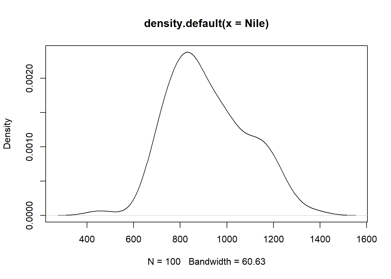
Exercise: 17-A
Create a density plot using the “Nile” dataset.
Answers
Answer: 15-A
Here’s how you can accomplish this task:
summary(mtcars)
      mpg             cyl             disp             hp
 Min.   :10.40   Min.   :4.000   Min.   : 71.1   Min.   : 52.0
 1st Qu.:15.43   1st Qu.:4.000   1st Qu.:120.8   1st Qu.: 96.5
 Median :19.20   Median :6.000   Median :196.3   Median :123.0
 Mean   :20.09   Mean   :6.188   Mean   :230.7   Mean   :146.7
 3rd Qu.:22.80   3rd Qu.:8.000   3rd Qu.:326.0   3rd Qu.:180.0
 Max.   :33.90   Max.   :8.000   Max.   :472.0   Max.   :335.0
      drat             wt             qsec             vs
 Min.   :2.760   Min.   :1.513   Min.   :14.50   Min.   :0.0000
 1st Qu.:3.080   1st Qu.:2.581   1st Qu.:16.89   1st Qu.:0.0000
 Median :3.695   Median :3.325   Median :17.71   Median :0.0000
 Mean   :3.597   Mean   :3.217   Mean   :17.85   Mean   :0.4375
 3rd Qu.:3.920   3rd Qu.:3.610   3rd Qu.:18.90   3rd Qu.:1.0000
 Max.   :4.930   Max.   :5.424   Max.   :22.90   Max.   :1.0000
       am              gear            carb
 Min.   :0.0000   Min.   :3.000   Min.   :1.000
 1st Qu.:0.0000   1st Qu.:3.000   1st Qu.:2.000
 Median :0.0000   Median :4.000   Median :2.000
 Mean   :0.4062   Mean   :3.688   Mean   :2.812
 3rd Qu.:1.0000   3rd Qu.:4.000   3rd Qu.:4.000
 Max.   :1.0000   Max.   :5.000   Max.   :8.000
Answer: 16-A
You can create your model with the following code:
lm <-lm(weight ~ Diet + Time, data = ChickWeight)summary(lm)
Call:
lm(formula = weight ~ Diet + Time, data = ChickWeight)

Residuals:
     Min       1Q   Median       3Q      Max
-136.851  -17.151   -2.595   15.033  141.816

Coefficients:
            Estimate Std. Error t value Pr(>|t|)
(Intercept)  10.9244     3.3607   3.251  0.00122 **
Diet2        16.1661     4.0858   3.957 8.56e-05 ***
Diet3        36.4994     4.0858   8.933  < 2e-16 ***
Diet4        30.2335     4.1075   7.361 6.39e-13 ***
Time          8.7505     0.2218  39.451  < 2e-16 ***
---
Signif. codes:  0 '***' 0.001 '**' 0.01 '*' 0.05 '.' 0.1 ' ' 1

Residual standard error: 35.99 on 573 degrees of freedom
Multiple R-squared:  0.7453,    Adjusted R-squared:  0.7435
F-statistic: 419.2 on 4 and 573 DF,  p-value: < 2.2e-16
Answer: 17-A
You can create your density plot with the following code: