plot(mtcars$mpg)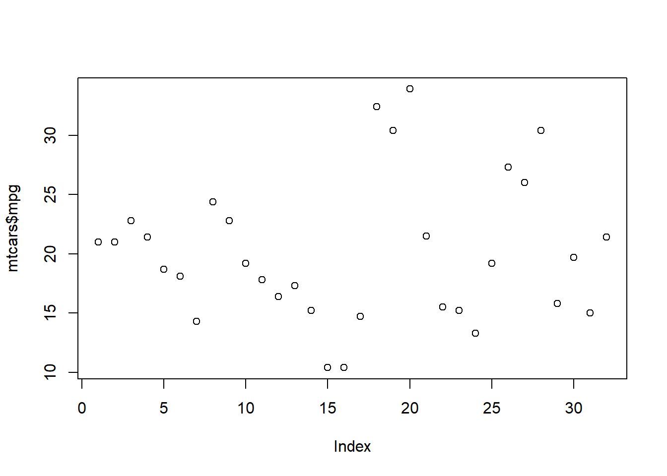
Outliers are observations that fall outside the expected scope of the dataset. It’s important to identify outliers in your data and determine the necessary treatment for them before moving into the next analysis phase.
For example, it might be necessary to impute values, remove a row, perform sensitivity analysis, or choose analysis methods that are robust in the presence of outliers.
One common first step many people employ when looking for outliers is visualizing their datasets so that extreme values can quickly be spotted This section will briefly cover several common visualizations used to identify outliers; however, each of these plots will be explored more in-depth later in the book.
This is probably the first plot you’ll reach for when trying to visualize outliers in your data. The scatter plot is a great tool to quickly visualize your data at a high level and see if anything major stands out.
plot(mtcars$mpg)
Here’s how a scatter plot with an extreme outlier might look.
data <- c(1,4,7,9,2,6,3,99,4,2,7,8)
plot(data)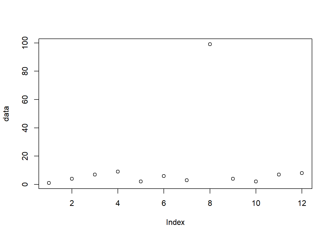
Another way to quickly visualize outliers is to use the “boxplot” function. This plot will allow you to evaluate outliers in a more systematic way.
boxplot(mtcars$mpg)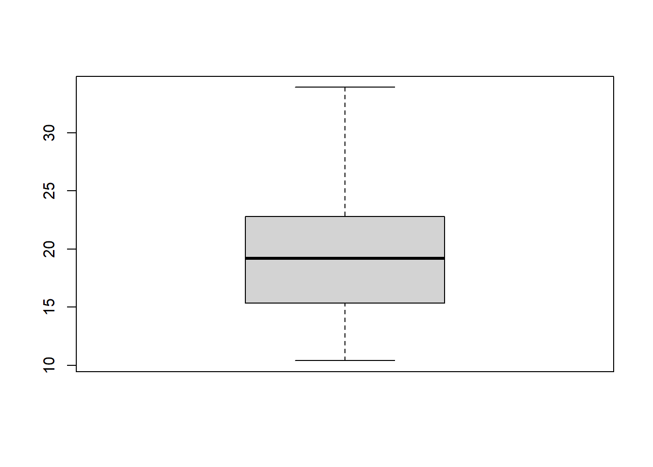
The solid black line represents the median value of your dataset. The top and bottom “whiskers” represent your extreme values (minimum and maximum). The top and bottom of the “box” represent the first and third quartile.
Here’s an example of a box plot with an extreme outlier.
boxplot(data)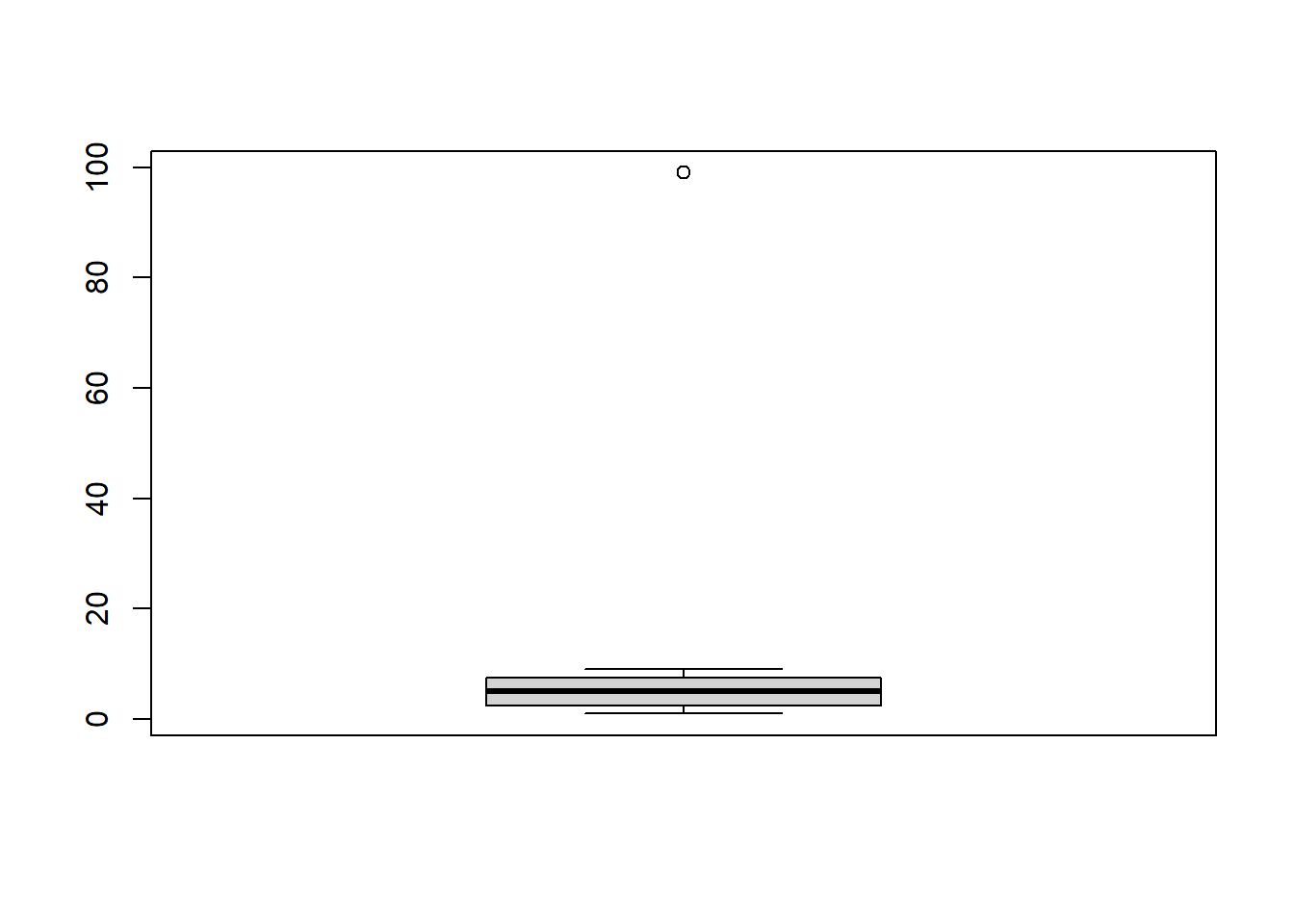
Histograms will allow you to see how often values occur within certain buckets.
hist(mtcars$mpg)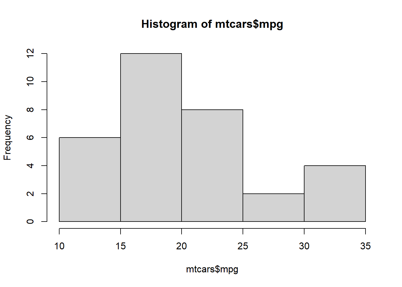
Here’s a histogram with data that contains an outlier.
hist(data)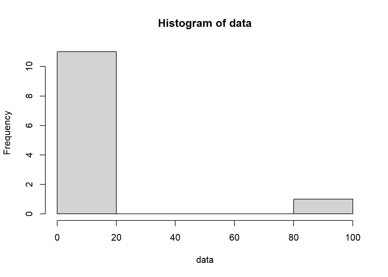
Density plots can be thought of as a smoothed version of a histogram. (You can tune the degree of smoothing, e.g. via the adjust argument to the density() function.)
plot(density(mtcars$mpg))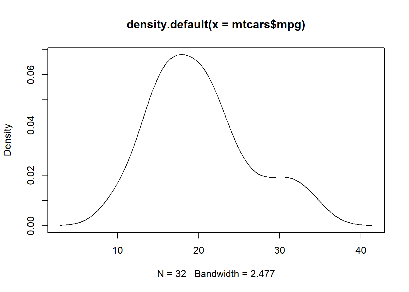
Here’s an example of a density plot with data that contains an outlier.
plot(density(data))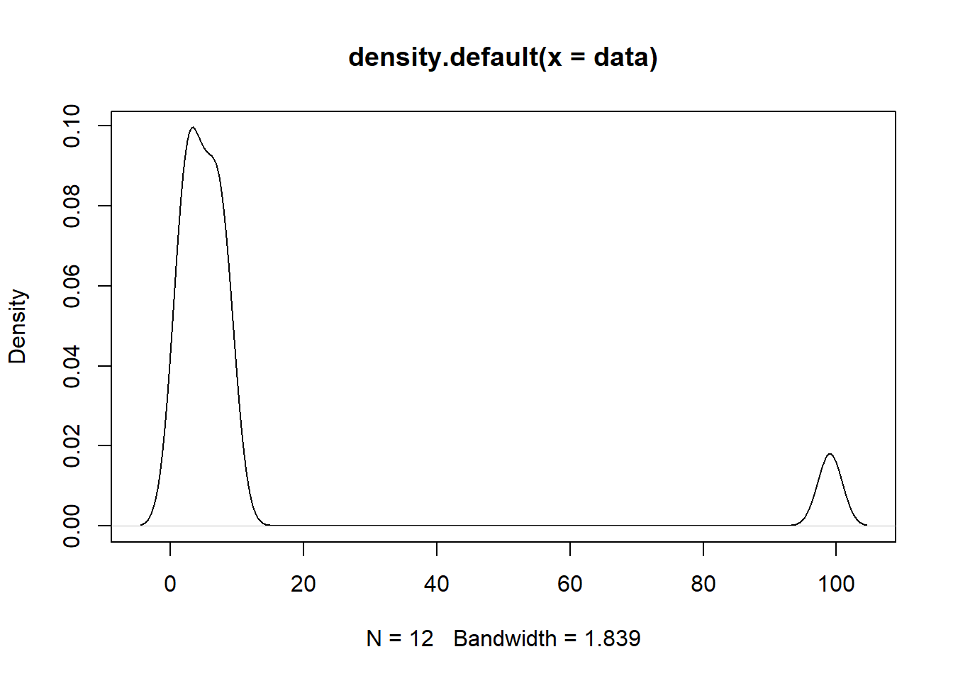
While examining your data visually may be a convenient and sufficient way to detect outliers in your data, sometimes you may require a more rigorous approach to outlier detection.
One simple way to check the extremity of your observation is to calculate how many standard deviations it falls from the mean.
Let’s start by calculating the standard deviation of our dataset by using the “sd” function.
sd <- sd(data)
print(sd)
[1] 27.31078Next, let’s calculate the mean of our dataset.
mean <- mean(data)
print(mean)
[1] 12.66667Finally, for each record in our vector, let’s calculate how many standard deviations it falls from the mean.
extremity <- abs(data - mean) / sd
print(extremity)
[1] 0.4271817 0.3173350 0.2074883 0.1342571 0.3905661 0.2441038 0.3539506
[8] 3.1611447 0.3173350 0.3905661 0.2074883 0.1708727After identifying your outliers you have several options to remove them.
Your first option would be to manually remove a specific outlier.
manually_cleaned <- data[data != 99]
print(manually_cleaned)
[1] 1 4 7 9 2 6 3 4 2 7 8A more robust option would be to rely on your previously performed calculations to remove any observations which are located too far away from the mean.
statistically_cleaned <- data[extremity < 3]
print(statistically_cleaned)
[1] 1 4 7 9 2 6 3 4 2 7 8“Statistics - Standard Deviation” by W3 Schools: https://www.w3schools.com/statistics/statistics_standard_deviation.php “Identifying outliers with the 1.5xIQR rule”: https://www.khanacademy.org/math/statistics-probability/summarizing-quantitative-data/box-whisker-plots/a/identifying-outliers-iqr-rule