5 Programming Basics
This chapter will walk you through executing code and writing scripts in R. You will then build upon that knowledge by learning about comments, variables, operators, functions, loops, conditionals, and libraries. While this chapter is titled “Programming Basics”, the knowledge you will have learned by the end of this chapter is enough for you to accomplish a huge variety of tasks.
5.1 Executing Code
When working in most programming languages, you will generally have the option to execute code one of two ways:
- in the console
- in a script
5.1.1 Console
The first way to run code is directly in the console. If you’re working in RStudio, you will access the console through the “console” pane.
Alternatively, if you downloaded R to your personal computer, you will likely be able to search your machine for an app named “RGui” and access the console this way as well.
In the following example, the text “print(3+2)”” is typed into the console. The user then presses enter and sees the result: “[1] 5”.
print(3+2)[1] 5You may be wondering what “[1]” represents. This is simply a line number in the console and can be ignored for most practical purposes. Additionally, most of the examples in this book will be structured in this way: formatted code immediately followed by the code output.
5.1.2 Script
You likely will be using scripts most of the time when working in R. A script is just a file that allows you to type out longer sequences of code and execute them all at once.
For those of you following along in RStudio, you can create a script by pressing “Ctrl + Shift + N” on Windows or by selecting “R Script” from the “New File” dropdown in the top left corner.
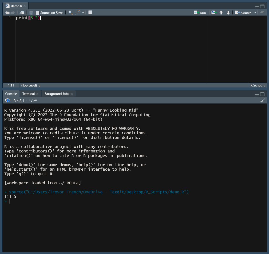
From here you can type the same command from before into the source pane. Next, you’ll want to save your file by pressing “Ctrl + S” on Windows or by selecting “Save” from the “File” dropdown in the top left corner. Now just give your file a name and your file will automatically be saved as a “.R” file.
Finally, run your newly created R script by pressing the “source” button.
5.3 Variables
Variables are used in programming to give values to a symbol. In the following example we have a variable named “rate” which is equal to 15, a variable named “hours” which is equal to 4, and a variable named “total_cost” which is equal to rate * hours.
rate <- 15
hours <- 4
total_cost <- rate * hours
print(total_cost)
[1] 605.4 Operators
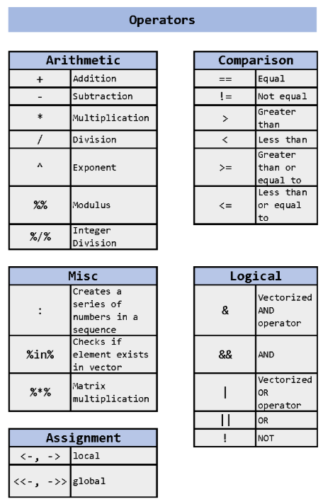
An operator is a symbol that allows you to perform an action or define some sort of logic. The following image demonstrates the operators that are available to you in R.
5.4.1 Arithmetic Operators
Arithmetic operators allow users to perform basic mathematical operations. The examples below demonstrate how these operators might be used. For those not familiar, the modulus operator will return the remainder of a division operation while integer (or Euclidean) division returns the result of a division operation without the fractional component.
3 + 3[1] 63 - 3[1] 03 * 3[1] 93 ^ 3[1] 2710 / 7[1] 1.42857110 %% 7[1] 310 %/% 7[1] 15.4.2 Comparison Operators
Comparison operators allow users to compare values. The examples below demonstrate how these operators might be used.
3 == 3[1] TRUE3 != 3[1] FALSE3 > 3[1] FALSE3 < 3[1] FALSE3 >= 3[1] TRUE3 <= 3[1] TRUE5.4.3 Logical Operators
Logical operators allow users to express “AND”, “OR”, and “NOT”. The following examples demonstrate how these operators might be used in conjunction with comparison operators as well as the difference between standard logical operators and “vectorized” logical operators.
In this example, we will evaluate two vectors of the same length from left to right. Each vector has seven observations (-3, -2, -1, 0, 1, 2, 3). Rather than simply returning a single “TRUE” or “FALSE”, this will return seven “TRUE” or “FALSE” values. In this case, the first element of each vector (“-3” and “-3”) will be evaluated against their respective conditions and return “TRUE” only if both conditions are met. This will then be repeated for each of the remaining elements.
# Vectorized "AND" operator
((-3:3) >= 0) & ((-3:3) <= 0)
[1] FALSE FALSE FALSE TRUE FALSE FALSE FALSEThis example will return a single “TRUE” only if both conditions are met, otherwise “FALSE” will be returned.
# Standard "AND" operator
(3 >= 0) && (-3 <= 0)
[1] TRUEThis example is the same as the previous one with the exception that we have negated the second condition with a “NOT” operator.
# Standard "AND" operator with "NOT" operator
(3 >= 0) && !(-3 <= 0)
[1] FALSEThe following two examples are essentially the same as the first two except that we are using “OR” operators rather than “AND” operators
# Vectorized "OR" operator
((-3:3) >= 0) | ((-3:3) <= 0)
[1] TRUE TRUE TRUE TRUE TRUE TRUE TRUE# Standard "OR" operator
(3 >= 0) || (-3 <= 0)[1] TRUE5.4.4 Assignment Operators
Assignment operators allow users to assign values to something. For most users, only “<-” or “->” will ever be used. These are called local assignment operators. However, there is another type of operator called a global assignment operator which is denoted by “<<-” or “->>”.
Understanding the difference between local and global assignment operators in R can be tricky to get your head around. Here’s an example which should clear things up.
First, let’s create two variables named “global_var” and “local_var” and give them the values “global” and “local”, respectively. Notice we are using the standard assignment operator “<-” for both variables.
global_var <- 'global'
local_var <- 'local'

global_var
[1] "global"local_var[1] "local"Next, let’s create a function to test out the global assignment operator (“<<-”). Inside this function, we will assign a new value to both of the variables we just created; however, we will use the “<-” operator for the local_var and the “<<-” operator for the global_var so that we can observe the difference in behavior.
Note
Functions are covered directly after this section. If the concept of functions is unfamiliar to you, feel free to jump ahead and come back later.
my_function <- function() {
   global_var <<- 'na'
   local_var <- 'na'
   print(global_var)
   print(local_var)
}

my_function()
[1] "na"
[1] "na"This function performs how you would expect it to intuitively, right? The interesting part comes next when we print out the values of these variables again.
global_var[1] "na"local_var[1] "local"From this result, we can see the difference in behavior caused by the differing assignment operators. When using the “<-” operator inside the function, it’s scope is limited to just the function that it lives in. On the other hand, the “<<-” operator has the ability to edit the value of the variable outside of the function as well.
You may now be wondering why both the local and the global assignment operators have two separate denotations. The following example demonstrates the difference between the two.
x <- 3
3 -> y

x
[1] 3y[1] 3There is also a third assignment operator that can be used: “=”. You will generally use the local assignment operator; however, you may notice that the “=” operator is used within certain functions as you progress. You can find more information about these three operators in the resources section.
5.4.5 Miscellaneous Operators
The “:” operator allows users to create a series of numbers in a sequence. This was demonstrated in the logical operator section. The %in% operator checks if an element exists in a vector. Both of these operators are demonstrated in the following example.
3 %in% 1:3[1] TRUEFinally, the “%*%” operator allows users to perform matrix multiplication as is demonstrated below. First, let’s create a 2x2 matrix and then let’s multiply it by itself.
x <- matrix(
  c(1,3,3,7)
  , nrow = 2
  , ncol = 2
  , byrow = TRUE)

x %*% x
[,1] [,2]
[1,] 10 24
[2,] 24 585.5 Functions
Functions allow you to bundle a predefined set of operations into one command. The syntax of functions in R is as follows.
# Create a function called function_name
function_name <- function() {
  print("Hello World!")
}

# Call your newly created function
function_name()
[1] "Hello World!"To go one step further, you can also add “arguments” to a function. Arguments allow you to pass information into the function when it is called. Here’s an example:
# Create a function called add_numbers which will add
# two specified numbers together and print the result
add_numbers <- function(x, y) {
    print(x + y)
}

# Call your newly created function twice with different inputs
add_numbers(2, 3)
[1] 5add_numbers(50, 50)[1] 100Finally, you can return a value from a function as such:
# Create a function called calculate_raise which multiplies
# base_salary and annual_adjustment and returns the result
calculate_raise <- function(base_salary, annual_adjustment) {
    raise <- base_salary * annual_adjustment
    return(raise)
}

# Calculate John's raise
johns_raise <- calculate_raise(90000, .05)

#Calculate Jane's raise
janes_raise <- calculate_raise(100000, .045)

print("John's Raise:")
[1] "John's Raise:"print(johns_raise)[1] 4500print("Jane's Raise:")[1] "Jane's Raise:"print(janes_raise)[1] 45005.6 Loops
There are two types of loops in R: while loops and for loops.
5.6.1 While Loops
While loops are executed as follows:
# Set i equal to 1
i <- 1

# While i is less than or equal to three, print i
# The loop will increment the value of i after each print
while (i <= 3) {
  print(i)
  i <- i + 1
}
[1] 1
[1] 2
[1] 3Additionally, you can add ‘break’ statements to while loops to stop the loop early.
i <- 1

while (i <= 10) {
    print(i)
    if (i == 5) {
        print("Stopping halfway")
        break
    }
    i <- i + 1
}
[1] 1
[1] 2
[1] 3
[1] 4
[1] 5
[1] "Stopping halfway"5.6.2 For Loops
For loops are executed as follows:
employees <- list("jane", "john")

for (employee in employees) {
  print(employee)
}
[1] "jane"
[1] "john"5.7 Conditionals
You are also able to execute a command if a condition is met by using “if” statements.
if (2 > 0) {
    print("true")
}
[1] "true"You can add more conditions by adding “else if” statements.
if (2 > 3) {
    print("two is greater than three")
} else if (2 < 3) {
    print("two is not greater than three")
}
[1] "two is not greater than three"Finally, you can catch anything that doesn’t meet any of your conditions by adding an “else” statement at the end.
x <- 20
if (x < 20) {
    print("x is less than 20")
} else if (x > 20) {
    print("x is greater than 20")
} else {
    print("x is equal to 20")
}
[1] "x is equal to 20"5.8 R packages
Packages allow you to access functions other people have created and shared in a standard format, e.g. via the Comprehensive R Archive Network (CRAN), Bioconductor, the r-universe or e.g. as github repositories.
To access a package’s functionality, you first have to add it to your system’s library. Afterward, you can check it out for use in your current session with the library() command.
In this example, we will be installing and loading a common package named “dplyr”.
You first retrieve it from CRAN with the following command.
install.packages("dplyr")Next, you make it available in your R session with the library() command. (Alternatively, you can also use the require() command.)
library(dplyr)You are now able to access all of the functions available in the dplyr library!
Sometimes users in the R community create their own packages that aren’t distributed through the CRAN network. You can still use these packages, but you’ll just have to perform an extra step or two. One of the most common places to host packages is Github. The following example will demonstrate how to load a package that I created from Github.
First you’ll need to install the “remotes” package. As the name might suggest, this package allows you to access other packages from remote locations.
install.packages("remotes")Next you’ll need to install the remote package of your choosing. In our case, we’ll execute the following code.
remotes::install_github("TrevorFrench/trevoR")In the previous example, we used the “install_github” function from the “remotes” package and then specified the Github path of the remote repository by typing “TrevorFrench/trevoR”. This code is functionally the same as the “install.packages” function. You may have noticed a new piece of syntax though. The “::” in between “remotes” and “install_github” tells R to use the “install_github” function from the “remotes” library without the need to require the library via the “library” function. This syntax can be used with any other function from any other library.
Now that the remote package is installed, we can require it in the same way we would any other package.
library(trevoR)5.9 Resources
- W3 Schools R Tutorial: https://www.w3schools.com/r/
- Assignment Operators: https://stat.ethz.ch/R-manual/R-devel/library/base/html/assignOps.html
5.2 Comments
Comments are present in most (if not all) programming languages. They allow the user to write text in their code that isn’t executed or read by computers. Comments can serve many purposes such as notes, instructions, or formatting.
Comments are created in R by using the “#” symbol. Here’s an example:
Some programming languages allow you a “bulk-comment” feature which allows you to quickly comment out multiple consecutive lines of text. However, in R, there is no such option. Each line must begin with a “#” symbol, as such:
Comments don’t have to start at the beginning of a line. You are able to start comments anywhere on a line like in this example: